R Programming: Beginner’s introduction on Data manipulation.
Skills
Author
Benjamini Mpinga
Published
April 25, 2023
R without data is just an Application. So to enjoy R programming then you need to deal with data. So in most cases you will be given data from outsource. And most of outsource data are not tidy, therefor you will need to tidy them before manipulation. Then you have to save them in your computer, tidy them, then model them, then share your findings. In R we use different approach when it comes to data manipulation, different from other languages, so once given data, the first thing to understand is its type.
The data below are not in tidy form, therefor we have to tidy them firstly. We will not write every step of the process because i believe you have already got the concept from the last lesson, but you can see the function in the chunk, we have equated our data by giving it a name raw. And followed by the name of extension, then my local directory and the name of the data.
require(tidyverse)
Loading required package: tidyverse
-- Attaching core tidyverse packages ------------------------ tidyverse 2.0.0 --
v dplyr     1.1.1     v readr     2.1.4
v forcats   1.0.0     v stringr   1.5.0
v ggplot2   3.4.2     v tibble    3.2.1
v lubridate 1.9.2     v tidyr     1.3.0
v purrr     1.0.1
-- Conflicts ------------------------------------------ tidyverse_conflicts() --
x dplyr::filter() masks stats::filter()
x dplyr::lag()    masks stats::lag()
i Use the conflicted package (<http://conflicted.r-lib.org/>) to force all conflicts to become errors
Loading required package: janitor

Attaching package: 'janitor'

The following objects are masked from 'package:stats':

    chisq.test, fisher.test
require(magrittr)
Loading required package: magrittr

Attaching package: 'magrittr'

The following object is masked from 'package:purrr':

    set_names

The following object is masked from 'package:tidyr':

    extract
require(readr)require(readxl)
How to tidy data 1st Example.
world population data before tidying.
popul=read.csv("e:/my_staffs/Blogs/teneson/posts/R-2nd-leson/The world population data/world_population.csv")
world population data after tidying.
popul=read.csv("e:/my_staffs/Blogs/teneson/posts/R-2nd-leson/The world population data/world_population.csv") %>%clean_names() %>%select(-c(2,4)) %>%pivot_longer(cols =4:11, names_to ="years", values_to ="populations") %>%mutate(years =replace(years, years =="x2000_population",2000), years =replace(years, years =="x2010_population",2010),years =replace(years, years =="x2015_population",2015),years =replace(years, years =="x2020_population",2020),years =replace(years, years =="x2022_population",2022),years =replace(years, years =="x1990_population",1990),years =replace(years, years =="x1980_population",1980), years =replace(years, years =="x1970_population",1970)) %>%rename(area.km.sq = area_km_a2) %>%rename(dens.km.sq = density_per_km_a2) %>%rename(percentage = world_population_percentage) %>%rename(growth.rate = growth_rate)
How to save tidy data.
popul %>%write.csv("clean_world_population.csv")
The data above show the raw data given from the original source which was collected and filed in csv extension, therefor in R programming language, you can’t work with data the same were collected in other orders. So as we have seen in above procedures, you will need to tidy them to be supported in R. and the above procedures are some of the few ways to deal with messy data you might come across with.
How to tidy data 2nd example.
raw =read_excel("e:/my_staffs/Blogs/teneson/posts/R-2nd-leson/Tamisemi/Primary Enrolment by Age and Sex,2021.xls")
So step 2, we are going to equate our data again and rename column, then remove column 1,28 and 29, because they provide no necessary information therefor we shall remain with 26 column. Now our data is called moja.We shall use function “clean names” of “Janitor package”.
moja = raw %>%clean_names() %>%select(-c(1,28,29))
Now let’s rename our 7 to 26 column because they are not well arranged, as we can see age and gender are both in same column, in order to put it easier for analysis, then we must separate them. But yet the data frame shows that ages of kids are not specified, some are actual and some are unspecific, therefore we are going to predict some values that can help in analysis, where age is below 6 we shall put 5, and where is above 13 we shall put 14, then we will specify in detail in an output. Here we shall use pivot function of janitor package which is in tidyverse package.
Now we deselect kids column and registration number column.
tatu = mbili %>%select(-c(5,7))
R Studio auto generated data.
We can also get data from R studio itself, Now lets jump strait to Rstudio on computer and see how you can get data, and see how to tidy data and share the results.
Temperature Data.
sample1 =rnorm(n =10, mean =26, sd =2) %>%as_tibble() %>%mutate(sample ="samp1")sample2 =rnorm(n =20, mean =26, sd =2) %>%as_tibble() %>%mutate(sample ="samp2")sample3 =rnorm(n =30, mean =26, sd =2) %>%as_tibble() %>%mutate(sample ="samp3")sample4 =rnorm(n =40, mean =26, sd =2) %>%as_tibble() %>%mutate(sample ="samp4")sample5 =rnorm(n =50, mean =26, sd =2) %>%as_tibble() %>%mutate(sample ="samp5")
Bind rows and columns.
How to bind different samples to a one data set, you either combine rows or columns. We use the function bind_rows/bind_col.
We have created different sample size and bind five samples together, we have used the function binding_rows to bind. We have named them (data.sample). But these data are auto-generated from the system, so they change from time to time as you run your chunk. Therefor in order to permanently use them without changes, then you’ll need to save them in your directory.
HOW TO SAVE AUTO GENERATED DATA TO YOUR COMPUTER.
When you import data into R, we use the function read_. But to save generated data from the system to local directory we apply the function write_, and you may save it in whatever extension you often use. Here under is the function plus application to save the data generated from the system in local directory. Our new data will be called datasample. We put a comment (#) so that a chunk not to run. still it show how it’s applicable in case you want to save your data.
#data.sample %>% write_csv("datasample.csv")
Now that our data are saved in our local directory, then to use it we must import in R. In importation we shall equate it as supa.
supa =read_csv("datasample.csv")
Rows: 150 Columns: 2
-- Column specification --------------------------------------------------------
Delimiter: ","
chr (1): sample
dbl (1): value

i Use `spec()` to retrieve the full column specification for this data.
i Specify the column types or set `show_col_types = FALSE` to quiet this message.
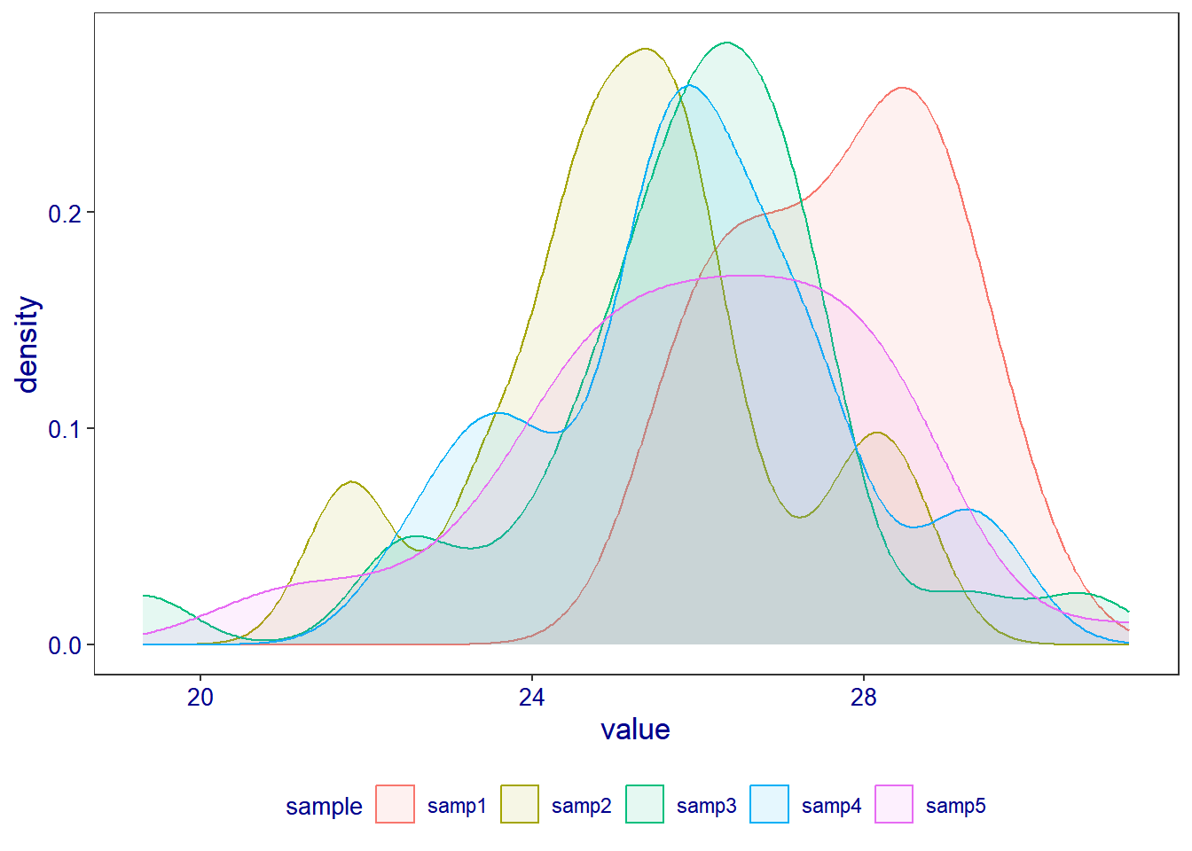
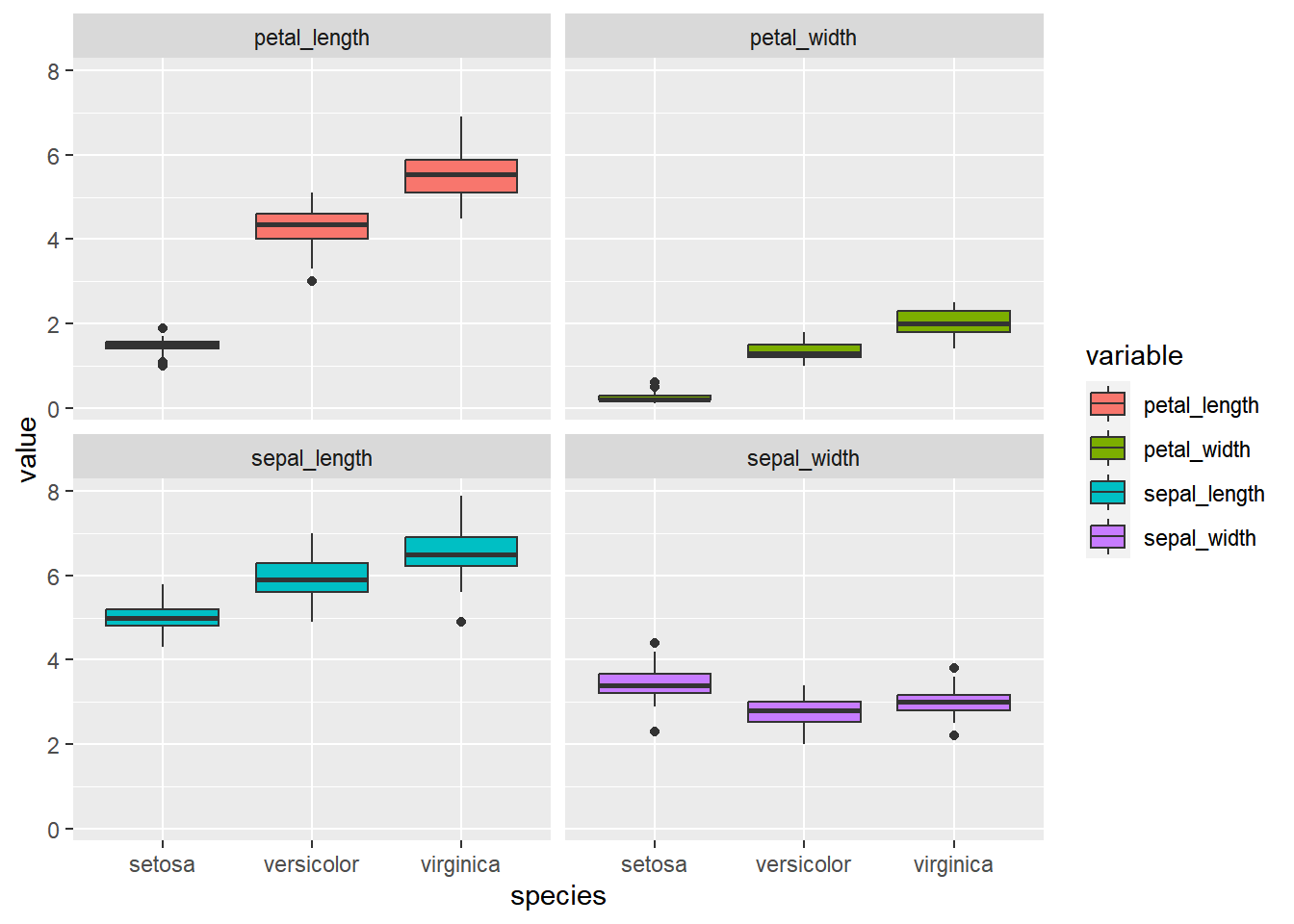
above figure show all sample’s result together, it is easier to present samples result in one figure, but the main purpose is to be understandable. Therefor it may be a bit harder for a viewer to understand the above figure. So in such situation we can opt to present our figure in separate samples.
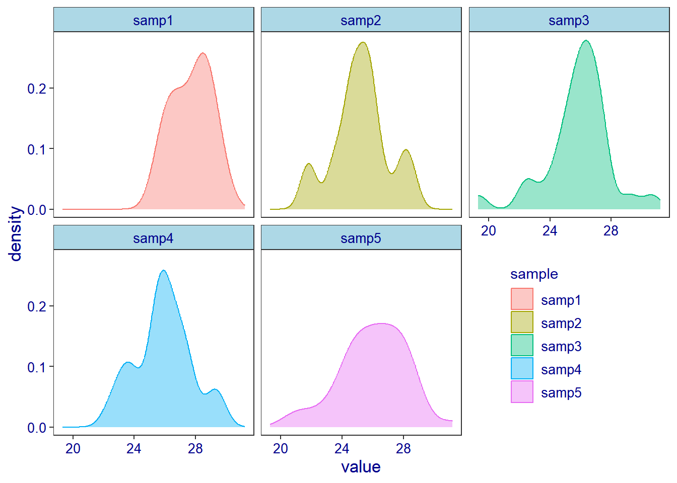
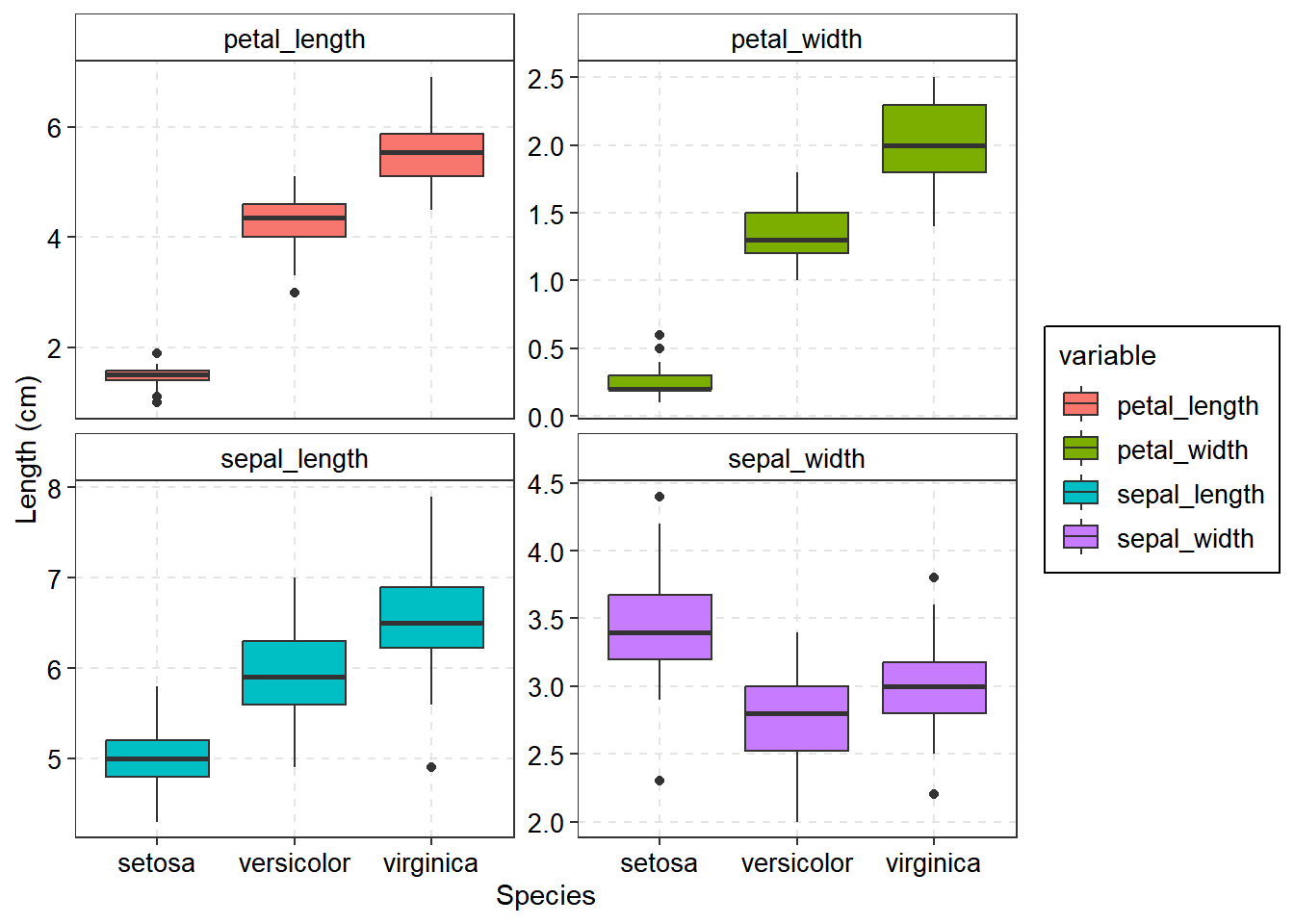
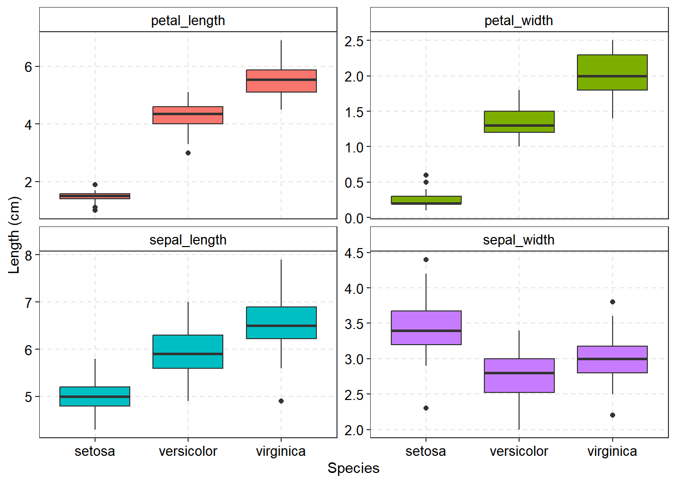
The above figure samples now are clearly observed. Also proves the concept that “you are in good position to get right result when you have enough sample”. Therefor you will need to consider the sample size before rushing to analysis.